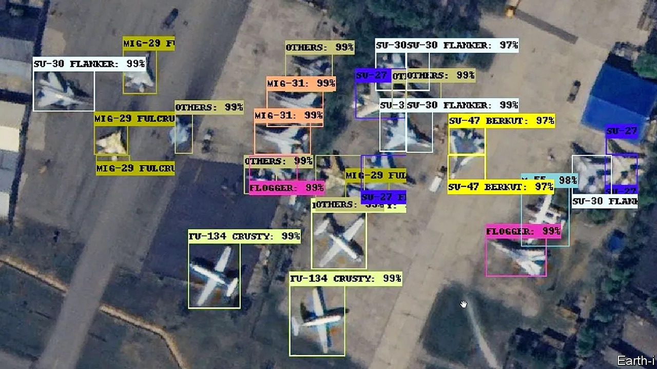
Satellite Imgae Classification

Recent advances in deep learning have enabled significant progress in computer vision tasks like image classification. One particularly interesting application is classifying satellite imagery, which has many real-world use cases from urban planning to environmental monitoring. In this post, I'll walk through my experience training and evaluating several popular convolutional neural network (CNN) architectures on the RSI-CB256 satellite image dataset.

The Dataset

The RSI-CB256 dataset contains 36,288 satellite images covering four different classes:

• Barren land
• Vegetation
• Water
• Construction

The images were sourced from remote sensing imagery as well as Google Maps snapshots, with each class containing a mix from both sources. At 256x256 pixels, the images are fairly high resolution, allowing the models to pick up on detailed textures and patterns.

Data Preparation

The RSI-CB256 dataset comes pre-organized with the images separated into four folders corresponding to the four classes: barren land, vegetation, water, and construction. This made it easy to use Keras' ImageDataGenerator to efficiently load images during training and evaluation.

I split the full dataset into 80% train, 10% validation, and 10% test sets using scikit-learn's train_test_split function. Then I created data generators for each split that could load images in batches, apply data augmentation, and preprocess the images on the fly:

def create_gens(train_df, valid_df, test_df, batch_size):
	img_size = (224, 224)
	channels = 3
	img_shape = (img_size[0], img_size[1], channels)
	ts_length = len(test_df)
	def scalar(img):
		return img
	tr_gen = ImageDataGenerator(preprocessing_function= scalar, horizontal_flip= True)

	ts_gen = ImageDataGenerator(preprocessing_function= scalar)
	train_gen = tr_gen.flow_from_dataframe( train_df, x_col= 'filepaths', y_col= 'labels', target_size= img_size, class_mode= 'categorical',
										color_mode= 'rgb', shuffle= True, batch_size= 40)
	valid_gen = ts_gen.flow_from_dataframe( valid_df, x_col= 'filepaths', y_col= 'labels', target_size= img_size, class_mode= 'categorical',
										color_mode= 'rgb', shuffle= True, batch_size= 40)
	test_gen = ts_gen.flow_from_dataframe( test_df, x_col= 'filepaths', y_col= 'labels', target_size= img_size, class_mode= 'categorical',
										color_mode= 'rgb', shuffle= False, batch_size= 40)
	return train_gen, valid_gen, test_gen

dir = '/kaggle/input/satellite-image-classification/data'

df = create_df(dir)
train_df, test_valid_df = train_test_split(df, test_size=0.2, random_state=42)
test_df, valid_df = train_test_split(test_valid_df, test_size=0.5, random_state=42)

# Get Generators
batch_size = 200
train_gen, valid_gen, test_gen = create_gens(train_df, valid_df, test_df, batch_size)
							

The key pieces in this code are:

• Defining an ImageDataGenerator for the training set that applies horizontal flips for basic data augmentation.
• Using flow_from_dataframe to generate batches, specifying the directory where the images are located.
• Setting parameters like target image size, color mode, shuffle, batch size, etc. Since the dataset was already split into separate class folders, the flow_from_dataframe method automatically loaded the images and associated labels correctly.

I resized the images to 224x224 pixels to match the default input size of the models I tested. Basic augmentation like horizontal flips helps prevent overfitting, though exploring more advanced augmentation could likely boost performance.

Model Architectures

I decided to test three well-known CNN model families that have shown strong performance on image classification tasks:

• EfficientNet: Developed by Google Brain, this model scales up existing architectures like MobileNets and achieves better accuracy and efficiency through compound scaling of dimensions like depth, width and resolution. I used the EfficientNetB0 variant.
• ResNet: The residual network architecture from Microsoft introduced skip connections to allow easier training of very deep networks (up to 152 layers in ResNet-152). I used the ResNet50 variant which is 50 layers deep.
• VGG: The VGG network from Oxford prioritizes depth over width, with very small 3x3 convolutional filters stacked to achieve a large effective receptive field. I used the VGG16 variant with 16 weight layers.

For each model, I used transfer learning by initializing the weights from an ImageNet pretrained model, then fine-tuning the full network on the RSI-CB256 dataset.
Here's an example of how I defined and compiled the EfficientNet model:

import tensorflow as tf
from tensorflow.keras.models import Sequential
from tensorflow.keras.layers import Dense, Dropout, BatchNormalization
from tensorflow.keras.callbacks import ModelCheckpoint

# Assuming train_gen and valid_gen are your image data generators

img_size = (224, 224)
channels = 3
img_shape = (img_size[0], img_size[1], channels)
class_count = len(list(train_gen.class_indices.keys()))

# Create pre-trained model
base_model = tf.keras.applications.EfficientNetB3(include_top=False, weights="imagenet", input_shape=img_shape, pooling='max')
for layer in base_model.layers:
    layer.trainable = False
model = Sequential([
    base_model,
    BatchNormalization(),
    Dense(256, activation='relu'),
    Dropout(0.3),
     Dense(64, activation='relu'),
    Dropout(0.3),
    Dense(class_count, activation='softmax')
])

optimizer = tf.keras.optimizers.Adam()
model.compile(optimizer=optimizer, loss='categorical_crossentropy', metrics=['accuracy'])

# Define filepath to save the best model
filepath = 'best_model.h5'

# Create ModelCheckpoint callback to save the best model based on validation accuracy
checkpoint = ModelCheckpoint(filepath, monitor='val_accuracy', verbose=1, save_best_only=True, mode='max')
# Train the model with the added callback
history = model.fit(
    x=train_gen,
    epochs=10,
    verbose=1,
    validation_data=valid_gen,
    callbacks=[checkpoint]
)
								

Training Details

I trained each model for 50 epochs with a batch size of 32 on Google Colab using freely available GPU resources. I used the RMSprop optimizer with a learning rate of 1e-4.
The training accuracy plots showed that all three models were able to achieve over 95% accuracy on the training set by the end of training. However, their performance differed on the held-out validation set:

Results Analysis

To evaluate the performance of the models on the test set, we can examine the confusion matrix which shows how often each class was correctly predicted versus misclassified.